Introduction
A neural network is a type of computer model that draws inspiration from the composition and operations of the human brain. It's a basic idea in artificial intelligence and machine learning, applied to problems including pattern recognition, clustering, regression, and classification.
How a neural network works:
1. Neurons: Artificial neurons, or nodes, are a neural network's fundamental building pieces. Every neuron receives several inputs, processes them, and then generates an output. An activation function is usually applied after the weighted sum of the inputs in the computation.
2. Layers: A neural network is composed of layers of neurons. There may be one or more hidden layers in between the input layer, which receives the raw input data, and the output layer, which generates the final output.
3. Connections: Neural connections, also known as weights, are used to indicate the intensity of the connection between two neurons in neighbouring layers. During the training phase, these weights are changed to maximise the network's performance for a particular job.
4. Activation Function: Each neuron typically applies an activation function to its weighted sum of inputs before passing the result to the next layer. Common activation functions include sigmoid, tanh, ReLU (Rectified Linear Unit), and softmax.
5. Feedforward Propagation: During the feedforward phase, input data is passed through the network layer by layer, with each layer performing its computations and passing the results to the next layer until the output is generated.
6. Backpropagation: This involves modifying the network's link weights in order to minimise the discrepancy between the expected and actual outputs. It entails figuring out a loss function's gradient in relation to the weights of the network and utilizing gradient descent or one of its variations to update the weights.
7. Training: The neural network is trained using a dataset with known inputs and outputs. During training, the network learns to map inputs to outputs by adjusting its weights through the process of backpropagation.
8. Evaluation: Once trained, the neural network can be evaluated on new, unseen data to assess its performance and generalisation ability.
Importance of Neural Networks:
1. Flexibility: Classification, regression, grouping, and generative modelling are just a few of the many tasks that neural networks can be used for due to their extreme flexibility. They can be used in a variety of fields, including speech recognition, picture identification, natural language processing, and more, thanks to their capacity to extract intricate patterns from data.
2. Feature Learning: The requirement for human feature engineering is eliminated by neural networks' ability to automatically extract pertinent features from raw data. They are therefore ideally suited for jobs where it is difficult or time-consuming to extract significant features.
3. Scalability: Neural networks can scale to handle large and complex datasets efficiently, thanks to advancements in hardware (such as GPUs and TPUs) and software frameworks (such as TensorFlow and PyTorch). This scalability enables the training of deep neural networks with many layers, which can capture intricate relationships in the data.
4. State-of-the-Art Performance: In many domains, neural networks have achieved state-of-the-art performance, surpassing traditional machine learning algorithms and even human-level performance in tasks such as image recognition, speech recognition, and game playing.
5. Adaptability to Unstructured Data: Text, audio, and picture data that is unstructured is a great fit for neural networks. While recurrent neural networks (RNNs) are better suited for sequential data like text and time series, convolutional neural networks (CNNs) are especially good at jobs involving spatial data like images.
6. Generalisation: Neural networks that have been trained properly frequently exhibit strong generalisation to new data, enabling them to generate precise predictions on brand-new, untested samples. The ability to generalise is essential for implementing machine learning models in practical settings.
7. Continuous Improvement: Neural network research is a rapidly evolving field, with ongoing advancements in architecture design, optimization techniques, and training algorithms. This continuous innovation drives improvements in model performance and efficiency.
8. Interpretability: There is continuous research on methods for comprehending and interpreting neural network predictions, despite the fact that neural networks are sometimes criticized for being harder to interpret than more straightforward models like decision trees. This covers techniques for displaying model internals, spotting key characteristics, and coming up with justifications for model choices.
Types of neural networks:
Feedforward Neural Networks (FNN):
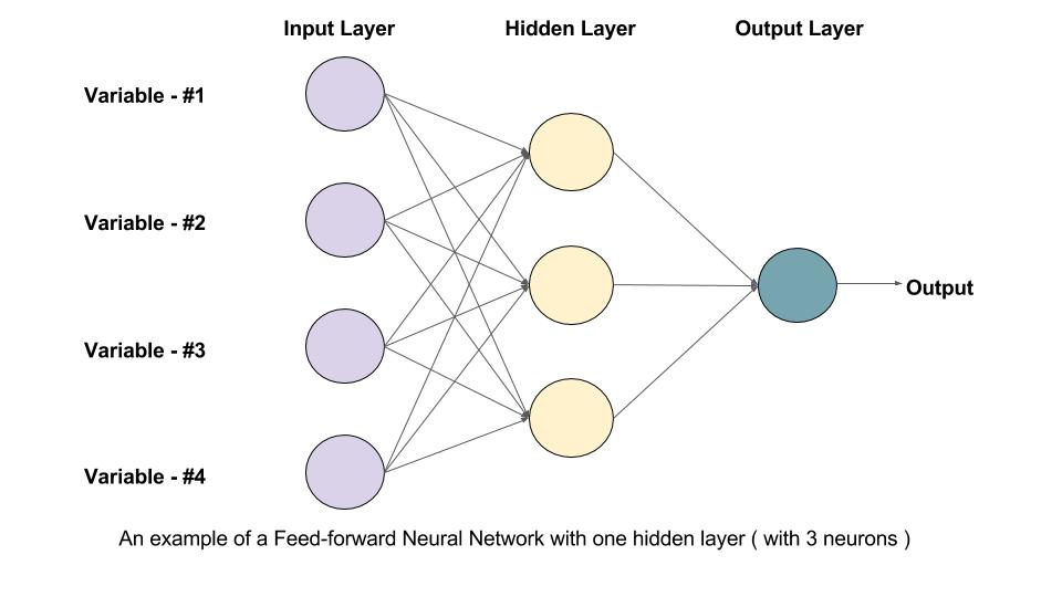
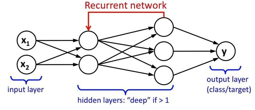
Multilayer Perceptrons, or Feedforward Neural Networks (FNNs), are a fundamental class of artificial neural networks. They are made up of an output layer, an input layer, and one or more hidden layers. Information moves from the input layer through the hidden layers and out to the output layer in FNNs in a single path.
1. Input Layer: The input layer consists of neurons, each representing a feature of the input data. Each neuron in the input layer is connected to every neuron in the subsequent hidden layer(s).
2. Hidden Layers: Between the input and output layers of a FNN, there may be one or more hidden layers. Neurons in each hidden layer process the input data through calculations. Hidden layer neurons add non-linearity into the network through activation functions, which helps the network recognize intricate patterns in the data. During model training, hyperparameters that must be adjusted include the number of hidden layers and the number of neurons in each layer.
3. Output Layer: The neural network's final predictions or outputs are generated by the output layer. The type of task determines how many neurons are needed in the output layer; for example, binary classification might need one neuron for a binary result, but multi-class classification might need many neurons, one for each class. Typically, an activation function suitable for the task—such as sigmoid for binary classification or softmax for multi-class classification—is applied by each neuron in the output layer.
4. Connections and Weights: Neurons in adjacent layers are connected by connections, each associated with a weight. These weights represent the strength of the connection between neurons and are adjusted during the training process to optimise the network's performance. The weights determine how much influence the output of one neuron has on the input of another neuron.
5. Activation Function: Each neuron (except those in the input layer) applies an activation function to the weighted sum of its inputs before passing the result to the next layer. Common activation functions include sigmoid, tanh, ReLU (Rectified Linear Unit), and softmax.
6. Training: FNNs are typically trained using backpropagation, a supervised learning algorithm. During training, the network learns to map inputs to outputs by adjusting its weights to minimise a loss function that measures the difference between predicted and actual outputs. Optimization techniques like gradient descent or its variants are used to update the weights iteratively.
Convolutional Neural Networks (CNN):
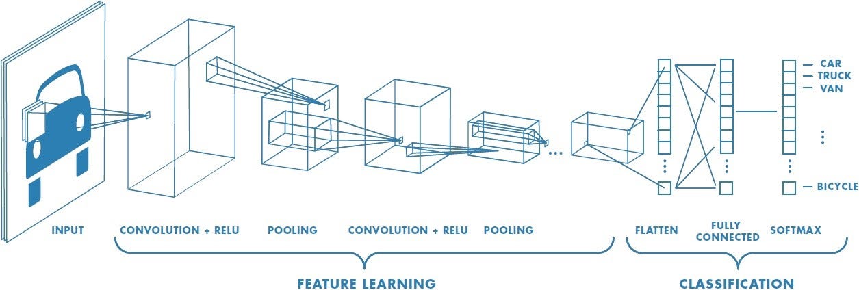
A specialised kind of neural network called a convolutional neural network (CNN) is made especially for processing data that resembles a grid, including pictures and movies. They have successfully been used in many other disciplines and have revolutionised the science of computer vision.
1. Convolutional Layers: Convolutional layers are CNNs' basic building components. To execute convolutions, these layers are made up of filters, also known as kernels, that slide over the input data, such as an image. For convolutions, the filter weights are multiplied element-by-element by the input data, and then the result is summated. Every convolution produces a feature map that draws attention to specific features or patterns in the input data. The input data is subjected to several filters, which produce a variety of feature maps, each of which captures a distinct component of the input.
2. Pooling Layers: The feature maps created by convolutional layers are downsampled using pooling layers, which lowers their spatial dimensions. Max pooling and average pooling are common pooling methods that preserve the maximum and average values in each pooling zone, respectively. Pooling lowers computational complexity and helps the network learn representations that are more resilient to changes in the input data.
3. Activation Functions: Activation functions, such as ReLU (Rectified Linear Unit), are typically applied after convolutions and pooling operations to introduce non-linearity into the network. ReLU is a popular choice due to its simplicity and effectiveness in combating the vanishing gradient problem.
4. Fully Connected Layers: At the end of the network, fully connected layers are frequently added in CNNs used for tasks like picture classification. Like classic feedforward neural networks, these layers link every neuron in one layer to every other layer's neuron. In fully connected layers, data from previous layers is combined to create the network's final output, which in the instance of picture classification is class probabilities.
5. Training and Backpropagation: Backpropagation is a supervised learning technique used in CNN training. The network learns to minimise a loss function—which calculates the difference between expected and actual outputs—during training. Recursive optimization methods such as Adam, RMSprop, or stochastic gradient descent (SGD) are employed to update the network's weights. Furthermore, methods such as batch normalisation and dropout can be used to enhance generalisation and convergence in training.
6. Transfer Learning: Through a process called transfer learning, CNNs trained on massive datasets such as ImageNet can be applied as feature extractors for other tasks. By leveraging the learned representations to achieve better performance with smaller training datasets, one can replace the fully connected layers of a pre-trained CNN with new layers specific to the target task.
Recurrent Neural Networks (RNN):
One type of neural network called recurrent neural networks (RNNs) is made to process data sequentially by preserving internal state or memory. RNNs can display temporal dynamic behaviour because they include connections that form directed cycles, in contrast to feedforward neural networks, which process input data in a single pass.
1. Recurrent Connections: The existence of recurrent connections, which enable information to endure over time, is what distinguishes RNNs. Every neuron in an RNN has a recurrent connection that links it to other neurons in the same layer or to itself at a prior time step. Recurrent neural networks (RNNs) are highly suited for applications like speech recognition, natural language processing, and time series prediction because they allow them to capture temporal dependencies in sequential data.
2. Internal State (Hidden State): RNNs preserve an internal state, sometimes referred to as the hidden state, at each time step that contains details about the input sequence that has been observed up to that point. The network may include data from earlier time steps into its predictions because the hidden state is updated recursively using the current input and the previous hidden state. Long-range dependencies in sequential data can be learned and remembered by RNNs thanks to the hidden state, which acts as a type of memory.
3. Sequence Processing: One element at a time, RNNs process sequential data, updating their hidden states iteratively and generating outputs at each time step. Sequences of any length can be fed into the network, and depending on the task at hand, RNNs can provide outputs of varying length. RNNs can handle sequences of different lengths, which makes them useful for applications like text production, sentiment analysis, and machine translation.
4. Vanishing Gradient Problem: Long-term dependency learning is hampered by RNNs' susceptibility to the vanishing gradient problem, in which gradients grow exponentially small during backpropagation through time (BPTT). Specialised RNN architectures, like Gated Recurrent Unit (GRU) networks and Long Short-Term Memory (LSTM) networks, have been created to address this problem. These structures have gating mechanisms that selectively regulate the information flow, making it easier for gradients to spread across lengthy sequences.
5. Training and Backpropagation Through Time (BPTT): The backpropagation through time (BPTT) technique, which is an extension of the backpropagation algorithm for feedforward neural networks, is commonly used to train RNNs. The network learns to minimize a loss function—which calculates the difference between expected and actual outputs—during training. In BPTT, the network is gradually unfurled into a directed acyclic graph (DAG), and gradients and weights are updated iteratively through the use of backpropagation.
Long Short-Term Memory Networks (LSTM):
Recurrent neural networks (RNNs) have problems when it comes to learning and remembering long-term dependencies in sequential data. To address these issues, LSTMs, a specialised sort of RNN architecture, were created. In 1997, Jürgen Schmidhuber and Sepp Hochreiter, introduced LSTMs.
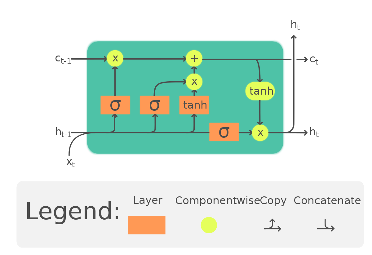
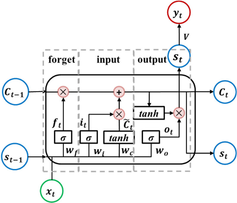
1. Memory Cells: LSTMs introduce a memory cell as the primary building block, allowing them to maintain long-term memory. The memory cell is responsible for storing information over extended time periods and selectively updating its content based on input and past information. The memory cell is regulated by three gates: the input gate, the forget gate, and the output gate.
2. Gates: Three different kinds of gates are used by LSTMs to control the information that enters and exits the memory cell: The input gate regulates how much fresh data should be added to the memory cell. The forget gate selects which data from the memory cell should be removed. The output gate controls how much data is sent to the network's output. Every gate uses sigmoid activation functions to generate an activation between 0 and 1 based on the inputs it receives, which include the current input, the prior concealed state, and maybe other context information. The amount of data that should pass through each gate is decided by these activations.
3. Cell State: Throughout the whole sequence, LSTMs preserve a distinct cell state in addition to the hidden state. The vanishing gradient issue that frequently befalls conventional RNNs is avoided by LSTMs thanks to the cell state, which enables them to store information over lengthy sequences. The input gate controls the selective addition of fresh data, the forget gate controls the removal of irrelevant data, and the output gate controls the exposure of pertinent data to the network's output. These processes update the cell state.
4. Activation Functions: LSTMs use various activation functions, including sigmoid and hyperbolic tangent (tanh), to control the flow of information and perform transformations on the input data and the cell state.
5. Training: LSTMs are trained using backpropagation through time (BPTT), an extension of the backpropagation algorithm for RNNs. During training, the network learns to minimise a loss function that measures the discrepancy between predicted and actual outputs. Gradients are computed using the chain rule and propagated backward through time, allowing the network to update its parameters (weights and biases) to improve performance.
Gated Recurrent Unit (GRU):
Another kind of recurrent neural network (RNN) architecture is the Gated Recurrent Unit (GRU), which was unveiled in 2014 by Kyunghyun Cho et al. GRUs are made to solve the vanishing gradient issue and identify long-term dependencies in sequential data, much as LSTMs. On the other hand, GRUs have fewer parameters and a simpler architecture than LSTMs
1. Update Gate and Reset Gate: The update gate controls the extent to which the past hidden state should be preserved and combined with the current input. The reset gate determines which parts of the past hidden state should be forgotten or reset based on the current input.
2. Hidden State: Like traditional RNNs and LSTMs, GRUs maintain a hidden state that evolves over time as the network processes sequential data. The hidden state captures the network's internal representation of the input sequence and encodes relevant information for making predictions.
3. Candidate Activation: In GRUs, the candidate activation is computed as a combination of the current input and the previous hidden state, similar to LSTMs. However, GRUs use different gating mechanisms compared to LSTMs to control the flow of information and update the hidden state.
4. Gating Mechanisms: The update gate and reset gate in GRUs are computed using sigmoid activation functions, producing values between 0 and 1. These gate values determine how much of the past hidden state and current input should be retained or forgotten when computing the candidate activation.
5. Hidden State Update: The updated hidden state is created by combining the prior hidden state with the candidate activation, which is managed by the update gate. GRUs can update the hidden state selectively while keeping pertinent historical data intact because of the update gate.
6. Training: Like classic RNNs and LSTMs, GRUs are trained by backpropagation through time (BPTT). The network learns to minimise a loss function during training by modifying its weights and biases in response to differences between expected and actual outputs. To iteratively update the network's parameters, gradients are computed using the chain rule and propagated backward through time.
Autoencoders:
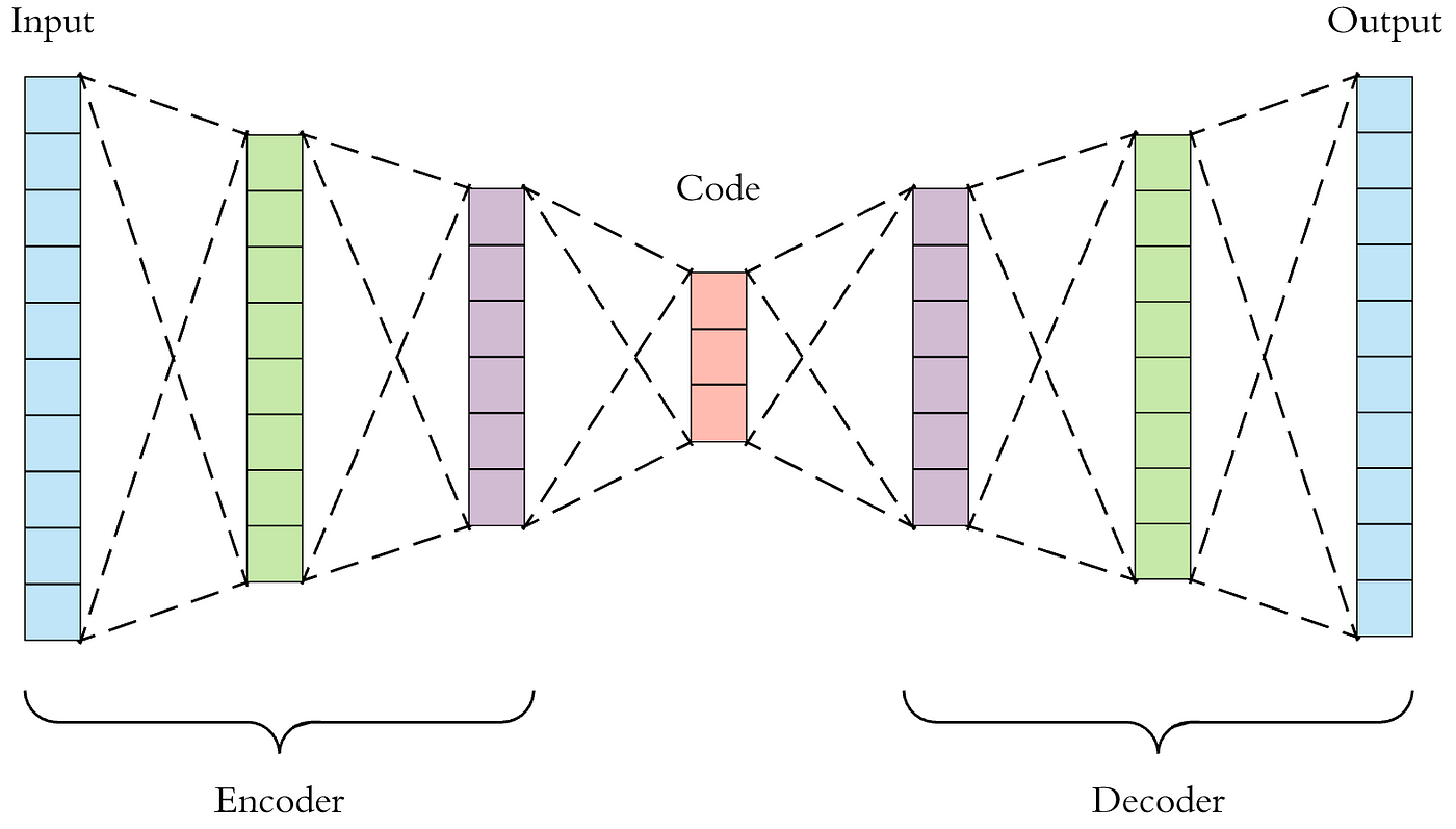
Neural networks using autoencoders are used for unsupervised learning, especially in feature learning, dimensionality reduction, and data compression applications. The basic principle of autoencoders is to minimise the reconstruction error by first learning a compact representation (encoding) of the input data and then reconstructing the original data from this representation (decoding).
1. Encoder: The initial part of an autoencoder is the encoder. It translates the input data to a representation in lower dimensions, often known as the latent space or encoding. Usually, the encoder is made up of one or more hidden layers that have a smaller number of neurons than the input layer. In order to add non-linearity, activation functions like sigmoid or ReLU are frequently utilised in the encoder's hidden layers.
2. Decoder: The second part of an autoencoder is the decoder. It translates the encoded representation—also known as latent space—that the encoder produced back to the initial input space. The architecture of the decoder and encoder are symmetric, with one or more hidden layers that progressively increase the dimensions until it returns to the initial input space. An activation function suitable for the type of input data is usually used by the decoder's output layer (e.g., sigmoid for binary data or linear for continuous data).
3. Latent Space: A lower-dimensional representation of the input data that the autoencoder has learned is called the latent space. Autoencoders are algorithms that take input data and encode it into a lower-dimensional space, allowing them to extract the important features or patterns from the data while removing noise and unnecessary information. One hyperparameter that must be selected depending on the trade-off between compression and reconstruction quality is the latent space's dimensionality.
4. Loss Function: In order to train autoencoders, a loss function measuring the difference between the input and reconstructed data is minimised. The kind of input data and the desired characteristics of the reconstructed output determine which loss function is used. For continuous data, mean squared error (MSE) is frequently utilised as the loss function; for binary data, binary cross-entropy is employed.
5. Training: Since autoencoders are trained by unsupervised learning, labelled data is not necessary for their training. Using optimization algorithms like gradient descent or its variations, the autoencoder learns to reconstruct the input data by minimising the reconstruction error during training. The network backpropagation reconstruction error, which modifies the weights of the encoder and decoder components.
6. Applications: Applications for autoencoders include feature learning, anomaly detection, data denoising, and dimensionality reduction. They can be employed as part of more intricate architectures for tasks like representation learning and picture production (e.g., variational autoencoders) or as a pre-train for deep neural networks.
Generative Adversarial Networks (GANs):
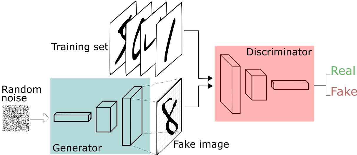
In 2014, Ian Goodfellow and associates proposed a new class of generative models called Generative Adversarial Networks, orGANs. The generator and discriminator neural networks, which make up GANs, are trained concurrently using a min-max game framework.
1. Generator: The generator creates synthetic data samples, including photos, depending on random noise that it receives as input. The generator's objective is to become proficient at creating data samples that are identical to actual data samples taken from the training distribution. Usually, the generator is made up of one or more hidden layers using sigmoid or ReLU activation functions.
2. Discriminator: Using samples of input data taken from the training set, the discriminator is a binary classifier that determines if the data is real or fake (produced by the generator). Accurately differentiating between authentic and fraudulent data samples is the discriminator's aim. Typically, the discriminator is made up of one or more hidden layers using sigmoid or ReLU activation functions.
3. Training Objective: In order to maximise competing objectives, the generator and discriminator of a GAN are trained simultaneously using a min-max game framework. The generator's goal is to reduce the likelihood that the discriminator will properly identify the samples it generates as fraudulent. On the other hand, the discriminator wants to be as good as possible in telling actual samples from fraudulent ones. Throughout the training process, the parameters of the discriminator and generator networks are updated iteratively in an effort to reach a Nash equilibrium, in which neither participant is able to unilaterally improve their strategy.
4. Loss Function: The binary cross-entropy loss, which gauges the discrepancy between the discriminator's predictions and the ground truth labels (actual or fake), is the source of the loss function used in GAN training. The binary cross-entropy between the discriminator's predictions for generated samples and a label signifying that they are real (even when they are phony) represents the generator's loss. The binary cross-entropy between the discriminator's predictions for created samples and a label indicating they are fake, as well as the binary cross-entropy between its predictions for genuine samples and a label indicating they are real, add up to the discriminator's loss.
5. Training Process: The discriminator and generator are alternately updated repeatedly in steps during training. Every time, a batch of synthetic samples is produced by the generator, and the discriminator is trained to discern between authentic and fraudulent samples. Subsequently, the generator is trained to produce samples that deceive the discriminator, hence enhancing its capacity to generate accurate data. Until the generator learns to produce samples that are almost identical to real data, this adversarial training process is repeated.
6. Applications: GANs have a wide range of applications, including image generation, style transfer, image-to-image translation, data augmentation, and super-resolution imaging. They have been used to generate realistic images of human faces, animals, landscapes, and other objects, as well as to create novel artwork and generate synthetic data for training machine learning models.
Transformers:
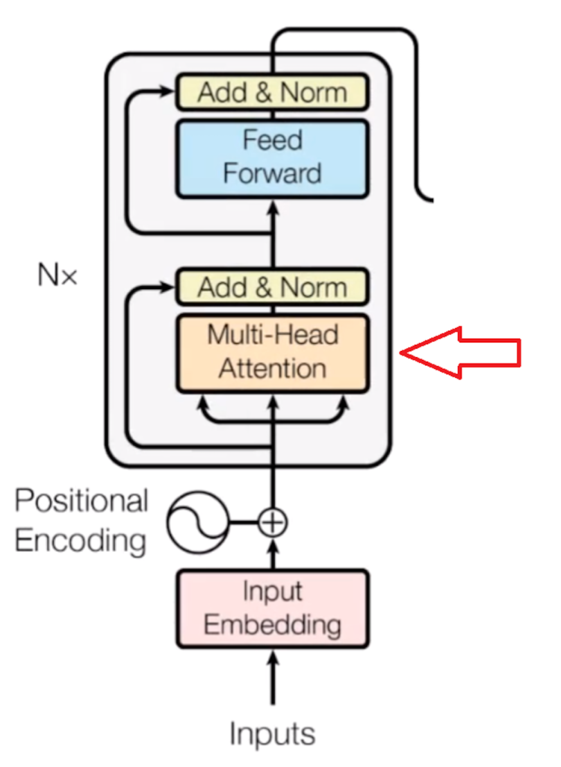
The 2017 research "Attention is All You Need" by Vaswani et al. introduced transformers as a kind of neural network design. Natural language processing (NLP) jobs have benefited greatly from transformers, which have also been used to a number of other domains than text.
1. Self-Attention Mechanism: Transformers' primary novelty is its self-attention mechanism, which enables the model to assess the relative significance of words in a sequence when encoding or decoding data. In order to capture interdependence between words regardless of their placements, self-attention computes attention ratings between all pairs of words in the sequence. Context-aware representations for every word in the sequence are created by computing the weighted sums of the input embeddings using the attention ratings.
2. Transformer Architecture: The encoder and decoder in the Transformer design are made up of several layers of feedforward and self-attentional neural networks. After processing the input sequence, the encoder creates a series of context-aware representations, which are then used by the decoder to create the output sequence. Layer normalisation and residual connections come after feedforward neural networks and self-attention as sub-layers in each of the encoder and decoder's layers.
3. Positional Encoding: Positional encoding is applied to the input embeddings to express the words' positions in the sequence, as transformers are not designed to capture word sequences naturally. The input embeddings are fed into the Transformer encoder after positional encodings have been applied. The relative positions of the words in the sequence are fed into the model by a variety of positional encoding approaches, including sine and cosine functions.
4. Multi-Head Attention: Transformers frequently use multi-head attention methods, in which several attention heads compute attention concurrently. The model is able to capture various features of the data because each attention head learns to focus on distinct portions of the input sequence. The final attention output is created by concatenating and linearly transforming the outputs of the several attention heads.
5. Position-wise Feedforward Networks: In addition to self-attention layers, Transformers include position-wise feedforward neural networks in each layer. These feedforward networks apply a series of linear transformations followed by non-linear activation functions (e.g., ReLU), processing each word's representation independently.
6. Training and Optimization: Typically, supervised learning is used to train transformers using large-scale datasets and goals like sequence-to-sequence modelling or maximum likelihood estimation. Transformer models are often trained using optimization methods like learning rate schedules and the Adam optimizer. Using self-supervised learning objectives like masked language modelling (e.g., BERT) or language modelling (e.g., GPT), transformers can be pre-trained on massive text corpora.
7. Applications: Transformers have achieved state-of-the-art results in various NLP tasks, including machine translation, text summarization, sentiment analysis, question answering, and named entity recognition. They have also been applied to other domains, such as image generation (e.g., Vision Transformer or ViT) and protein folding prediction.
Conclusion:
Computer vision, natural language processing, speech recognition, and many other industries have been transformed by neural networks, a potent family of machine learning models. Neural networks' capacity to extract intricate patterns and representations from data has made major strides possible in the solution of difficult issues that were previously thought to be unsolvable. navan.ai has a no-code platform - nstudio.navan.ai where users can build computer vision models within minutes without any coding. Developers can sign up for free on nstudio.navan.ai
Want to add Vision AI machine vision to your business? Reach us on https://navan.ai/contact-us for a free consultation.